Getting the Data
All the raw data used in our approach is inside the folder RawData folder. To access that folder you can run the following command in the terminal:
cd ~/Artifact/RawData
Directory Structure
This section will describe how the RawData directory is structured, formatted, and named. The directory is structured and shown in the image below (Note: the output of tree -d -L 4 --filelimit=10 has been edited somewhat for easier viewing on a website). The directory is separated into 5 folders. One folder FinalScoringModels contains the scoring model described later on this page. The other 4 folders that represent the main experiments that were run. The experiment folders have subfolders that represent the different test suites generated for each experiment. Inside each of these subfolders is a folder that contains each of the test cases, named maps.
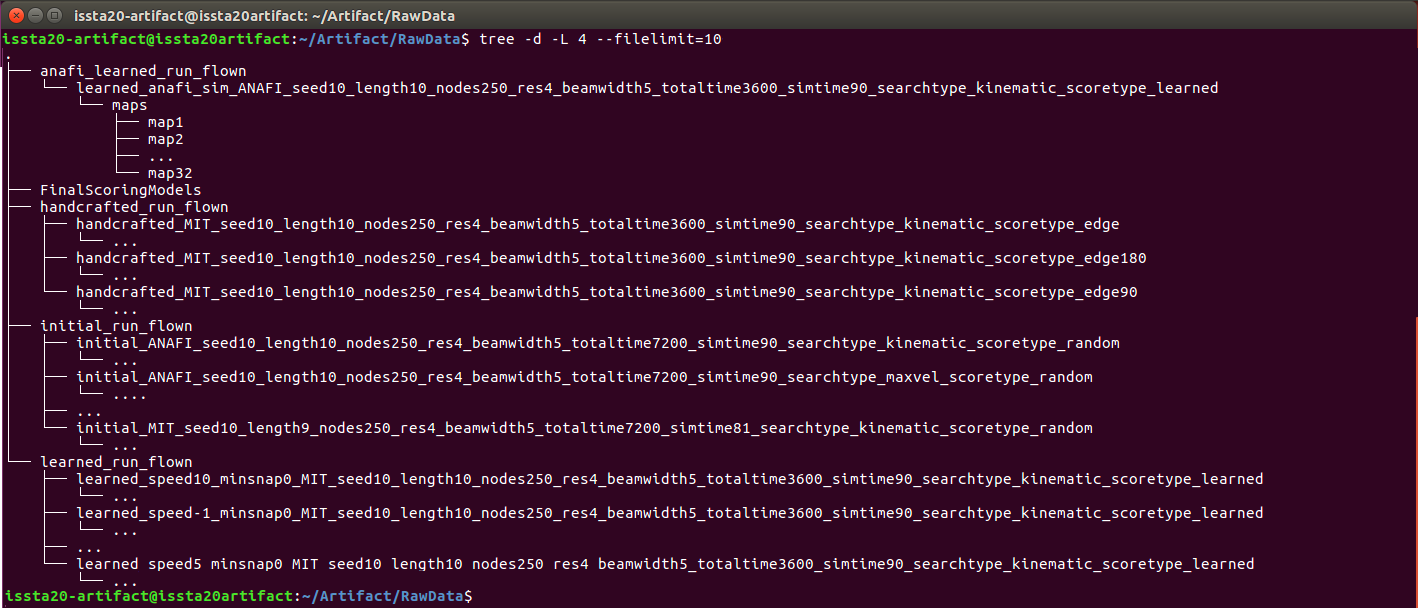
The 4 main experiments represent each of the different experiments that were run for our study. The experiments are named as follows
- initial_run_flown: This folder contains the initial tests suite that was generated for both the Anafi drone and the MIT Flightgoggles drone. It contains the tests generated using random selection, maximum velocity selection, as well as kinematic and dynamic selection. No scoring functions are used in any of these test suites.
- handcrafted_run_flown: This folder contains the test suite created using the handcrafted scoring models. These tests were only run on the MIT Flightgoggles drone.
- learned_run_flown: This folder contains the test suite generated for learned scoring models. There is a different scoring model for each of the MIT Flightgoggles drone controllers.
- anafi_learned_run_flown: This folder contains the test data for the learned scoring model of the Anafi drone.
We can view these folders by running an ls command in the RawData directory in our terminal, as shown below:

In the subsequent sections below, we give more details on the naming schemes, structure, and data contained inside each of the folders.
Test Suites
Each of the folders contains the test suites generated for that specific experiment. Below is a description of the test suite naming convention that was used. Each experiment folder contains a list of text file and folder pairs. The text files contain the terminal output created when running the test generation tool. The folders contain the actual test cases for each test suites. The folders and text file pairs were named using the test generation parameters.
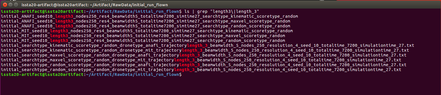
So, for instance, considering the text file below:
initial_searchtype_kinematic_scoretype_random_dronetype_anafi_trajectorylength_3_beamwidth_5_nodes_250_resolution_4_seed_10_totaltime_7200_simulationtime_27.txt
We can infer it was generated using the following parameters:
- Prefix (initial): A developer given prefix for the file name giving as a parameter to the test generation technique
- Search type (kinematic): The type of search model used. The model can be either no scoring model (random), an approximation of the scoring model using the maximum velocity (maxvel), or the kinematic and dynamic model (kinematic).
- Score type (random): The type of scoring model used. The scoring model can either be random, learned, or a custom name given to the type of handcrafted scoring technique.
- Drone Type (anafi): The type of physical drone used. In our studies, we targeted two physical drones, namely the Anafi drone (anafi) and MIT Flightgogggles drone (mit).
- Trajectory Length (3): The number of waypoints in a trajectory. This includes the start and end waypoint.
- Beam width (5): The size of the beamwidth used by the beam search algorithm.
- Nodes (250): The number of nodes in the world. Each node is a waypoint the drone may use to build its trajectory.
- Resolution (4): The number of linearly spaced input samples used. All permutations of each input linearly sampled values is used to compute all possible future states the quadrotor might attain.
- Seed (10): The seed used by the random generator.
- Total time (7200): The total time in seconds for test generation and testing the drone.
- Simulation time (27): The total time in seconds given to the simulator or outdoor test runs. This time is used by the test generation technique to take into account how much time is required to execute an identified test.
A very similar naming technique is used for the associated folder that contains the generated tests. For example, the above output file saved all the test cases inside the folder:
initial_ANAFI_seed10_length3_nodes250_res4_beamwidth5_totaltime7200_simtime27_searchtype_kinematic_scoretype_random
Using the naming convention, we can identify specific test suites we are interested in. Say, for instance, you want all test sets of length 3. We can find these test sets using the ls command and grep for any files or folders with length 3 in the ~RawData/initial_run_flown/ directory:
Individual Test Cases
Inside each of the test suites folders, you will find a set of individual test cases. The test cases are saved inside the maps folder. The maps folder contains all the test cases for that specific test suite. Each map is a unique test case which the robot could execute. If we were to run the ls command inside the maps folder, we would see the individual test cases. Selecting the first test case maps1 we can again use the ls command to see what each test contains:
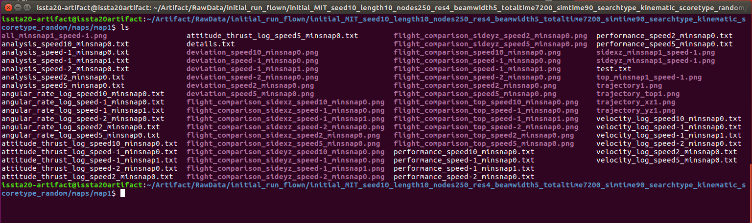
Each of the test cases contains a variety of data. We will now explain the data found inside each test case.
Generated Test
The files related to test generation are inside are described below:
| Name | Description |
|---|---|
| details.txt | Contains all the details of the test. These details include the save_location, the score given to the trajectory based on the scoring model used, the waypoints in the trajectory. The velocities required at each waypoint, the attitude required at each waypoint, the expected output and input velocities vectors for each waypoint, and the Euler angles to the next waypoint. |
| test.txt | The test file used by a simulator. The contains the waypoints for the test, the expected velocities, and a description of the environment (not used in this paper) |
| trajectory_top#.txt | An image showing the trajectory from a top view. # represents the test number. |
| trajectory_xz#.txt | An image showing the trajectory from a side view along the x-axis. # represents the test number. |
| trajectory_yz#.txt | An image showing the trajectory from a side view along the y-axis. # represents the test number. |
| trajectory#.txt | An image showing the 3D representation of the trajectory. |
Test Execution Data
If a test is executed, the resulting files are saved in the test case folder. Each of the resulting files is described below. The tests could be executed by the Anafi drone or the Flightgoggles MIT drone, which have different controllers. To easily identify the controller used, the following naming conventions were used:
| Name | Description |
|---|---|
| anafi | The data from the Anafi controller |
| speed-2_minsnap0 | The data from the unstable waypoint controller |
| speed-1_minsnap0 | The data from the waypoint controller |
| speed-1_minsnap1 | The data from the minimum snap controller |
| speed2_minsnap0 | The data from the fixed velocity controller attempting to maintain 2m/s |
| speed5_minsnap0 | The data from the fixed velocity controller attempting to maintain 5m/s |
| speed10_minsnap0 | The data from the fixed velocity controller attempting to maintain 10m/s |
When the test was run, they produced the following output that is also saved inside the test case folder (Note: {controller} can be replaced with any of the above-listed controllers).
| Name | Description |
|---|---|
| performance_{controller}.txt | The main data file which contains the current drones position, current goal, distance to the goal, and elapsed time. |
| angular_rate_log_{controller}.txt | A data file that contains the output of the angular rate controller. This includes the message publishing time, the angular rates in the X, Y, and Z direction as well as the thrust. |
| attitude_thrust_log_{controller}.txt | A data file that contains the output of the attitude and thrust controller. This includes the message publishing time, the requested attitude in the X, Y, and Z orientation as well as the thrust. |
| velocity_log_{controller}.txt | A data file that contains the output of the velocity controller. This includes the message publishing time, the requested velocity in the X, Y, and Z direction. |
There was one exception to this, namely the minimum snap controller. Due to the minimum snap controller computing its own curved trajectory through the waypoints when the minimum snap controller was executed, a few additional output files were generated for this controller. These files contained descriptions of the expected trajectory and are listed below:
| Name | Description |
|---|---|
| all_minsnap1_speed-1 | An image showing a 3D representation of the original trajectory and the computed minimum snap trajectory. |
| top_minsnap1_speed-1 | An image showing a top view of the original trajectory and the computed minimum snap trajectory. |
| sidexz_minsnap1_speed-1 | An image showing the side view along the x-axis of the original trajectory and the computed minimum snap trajectory. |
| sideyz_minsnap1_speed-1 | An image showing the side view along the y-axis of the original trajectory and the computed minimum snap trajectory. |
Analysis Data
After executing a test case, the performance was analyzed and output saved inside the test case folder. More details on the processing of the data can be found inside the Tool Pipeline section. However, for completion, a brief description of of the output files generated from processing is given below:
| Name | Description |
|---|---|
| analysis_{controller}.txt | A file that contains all the information extracted from the raw data. This includes the analysis of timing between waypoints, analysis of the deviation from the optimal trajectory, and analysis of the velocity and acceleration of the quadrotor. |
| deviation_{controller}.txt | An image showing the deviation from the optimal trajectory between waypoints. |
| flight_comparison_{controller}.txt | An image showing a 3D representation comparing the expected trajectory to the actual trajectory |
| flight_comparison_top_{controller}.txt | An image showing a top-down representation comparing the expected trajectory to the actual trajectory |
| flight_comparison_sidexz_{controller}.txt | An image showing a side view along the x-axis representation comparing the expected trajectory to the actual trajectory |
| flight_comparison_sideyz_{controller}.txt | An image showing a side view along the y-axis representation comparing the expected trajectory to the actual trajectory |
Scoring Models
The scoring models used in our study can be found in the ~Artifact/RawData/FinalScoringModels folder. The final models are the scoring models that were learned using the scikit-learn. For example, to list all the models, we can run the ls command to get the following output:
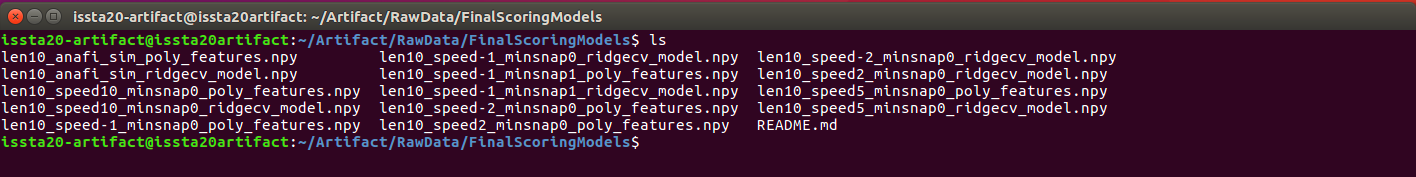
Looking at two of the models we see, they are named as follows.
len10_speed2_minsnap0_poly_features.npy
len10_speed2_minsnap0_ridgecv_model.npy
The naming scheme corresponds to the following:
- Trajectory Length (10): The number of waypoints in a trajectory. This includes the start and end waypoint.
- Controller type (speed2_minsnap0): The type of controller for which the model was generated.
- poly_features: The polynomial regression model.
- ridgecv_model: The ridge regression model.
Example: Using the Data
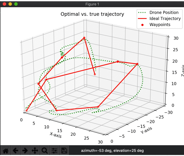
The full set of scripts used to process the data is made available in the Reproducing Results section. However, here is a basic example of how to use raw data to get something meaningful. Let’s say we wanted to visualize the experiment run on the learned scoring model of the MIT drone using a waypoint controller. We would navigate to the following folder:
cd ~/Artifact/RawData/learned_run_flown/learned_speed-1_minsnap0_MIT_seed10_length10_nodes250_res4_beamwidth5_totaltime3600_simtime90_searchtype_kinematic_scoretype_learned/maps/map1
Looking at the raw data in performance_speed-1_minsnap0.txt we would see the following data:
Goal switch
Time between goals: 0.011458337
Total Time: 0.011458337
-------------------------------
Current Drone Position: 2.03107024406e-05, -2.02185673403e-05, 1.49196065511
Current Goal Position: 0.1, -0.1, 0.1
Distance to Goal: 1: 1.3991234257
Elapsed Time: 0.100000032
-------------------------------
Current Drone Position: 0.000519302253194, -0.000511546461687, 1.46423436157
Current Goal Position: 0.1, -0.1, 0.1
Distance to Goal: 1: 1.3714699249
Elapsed Time: 0.200000064
-------------------------------
Current Drone Position: 0.00241670698523, -0.00236139983197, 1.42563186128
...
To make more sense of this data, we could write a small python script to parse it and display the Drone position and the Goal position.
import numpy as np
import matplotlib.pyplot as plt
from mpl_toolkits.mplot3d import Axes3D

def get_numbers_from_string(string_var):
    # Split by space
    space_list = string_var.split(" ")
    # Saves numbers
    final_numbers = []
    # Try convert each word to a number
    for s in space_list:
        # Remove comma
        s = s.strip(",")
        s = s.strip("[")
        s = s.strip("]\n")
        try:
            number = float(s)
            final_numbers.append(number)
        except:
            pass
    return final_numbers

# Used to store current test information
current_drone_position = []
test_waypoints = []
current_waypoint_position = []

# Initialize a dummy waypoint
waypoint = [-np.inf, -np.inf, -np.inf]

# Open the file
f = open("performance_speed-1_minsnap0.txt", "r")

for line in f:
    # Find the goal positions
    if "Current Goal Position" in line:
        goal_pos = get_numbers_from_string(line)
        current_waypoint_position.append(goal_pos)
        if goal_pos != waypoint:
            waypoint = goal_pos
            test_waypoints.append(waypoint)
    # Find the drone positions
    if "Current Drone Position" in line:
        current_position = get_numbers_from_string(line)
        current_drone_position.append(current_position)
f.close()

# Stack the drone positions and waypoints for plotting
d_pos = np.vstack(current_drone_position)
w_pos = np.vstack(test_waypoints)

# Create a 3D plot of the trajectory and actual path
fig = plt.figure()
ax = Axes3D(fig)
ax.plot3D(d_pos[:, 0], d_pos[:, 1], d_pos[:, 2], color='green', linestyle=":", linewidth=2, label='Drone Position')
ax.plot(w_pos[:, 0], w_pos[:, 1], w_pos[:, 2], color='red', linestyle="-", linewidth=2, label='Ideal Trajectory')
ax.scatter(w_pos[:, 0], w_pos[:, 1], w_pos[:, 2], c='red', label='Waypoints')
ax.set_xlim([0, 30])
ax.set_ylim([0, -30])
ax.set_zlim([0, 30])
ax.set_xlabel('X-axis')
ax.set_ylabel('Y-axis')
ax.set_zlabel('Z-axis')
plt.title("Optimal vs. true trajectory")
ax.legend()
plt.show()
The output of this script would create a 3D graph showing both the drones’ simulated motion as well as the expected trajectory.